2-D Mach 3 step test

This is another example of complex boundary conditions. A Mach 3 flow is forced through a constriction in the form of a step that narrows a rectangular 2-D pipe.

Using Fyris, it is relatively simple to implement the non-rectangular boundaries, using a set of smaller rectangular zones that are joined at their common boundaries. The upper and lower boundaries of the simulation are reflecting, including the leading edge of the step. The inlet on the left is held constant, and the outlet on the right is allowed to be a free boundary. The general geometry is seen in below.

The problem parameters are:

Adiabatic index: gamma = 1.4.
Grid domain: 0.0 < x < 3.0, 0.0 < y < 1.0
Step region: 0.2 < x < 3.0, 0 < y < 0.2
Initial grid values, v = 3.0, P = 1.0, d = 1.4
Left boundary: fixed inlet, v = 3.0
Right boundary: free outlet
All other boundaries: reflecting
Time limit: t = 4.0.

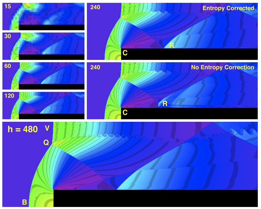
This simulation is discussed in detail in Collella & Woodward (1984), and in particular the treatment of the flow adjacent to the reflecting corner ( Cin the figure), is described. Essentially a correction is required in order to produce the correct entropy levels in cells adjacent to the corner. If not implemented correctly the boundary layer downstream from the corner is incorrect and the Reflection point ( marked by R) is disrupted. The two h= 240 panels in the figure shows the result of turning off the entropy correction.

Otherwise the simulation is sensitive to the accuracy of striping control used, especially at the leading edge of the curved bow shock ( B ) and in the nearly stationary strong vertical shock ( V ). Also, minute oscillations at the quadruple point ( Q ) provides stimulation to KH-waves on the slip line from that point. High resolution lagrangian methods like Fyris capture the formation of the KH-waves very well.